Simulating a bosonic error correcting code using Bosonic Qiskit

In a previous post on the Qiskit Medium, we introduced Bosonic Qiskit, an open-source project in the Qiskit ecosystem that allows users to construct, simulate, and analyze quantum circuits that contain bosonic modes (also known as oscillators or qumodes) alongside qubits. Now, we’re following up on that work with a closer look at one of the most promising applications of hybrid qubit-bosonic hardware: bosonic error correction.

Bosonic error correction is an error handling strategy in which logical qubits are encoded into the infinite-dimensional Hilbert space of a type of quantum system known as the quantum harmonic oscillator. Much like the quantum systems we use to encode qubits, a quantum harmonic oscillator has discrete or “quantized” energy levels. However, qubits have only two energy levels while oscillators are formally described as having infinite levels, a quality that offers key advantages for applications like quantum error correction. Physical realizations of quantum harmonic oscillators include the electromagnetic modes of a microwave cavity and the vibrational modes of a chain of ions, to name a few examples.

In this article, we will demonstrate the utility of Bosonic Qiskit for exploring this promising approach to quantum error correction through an explicit, tutorial-style demonstration of one of the simplest bosonic error correction codes — the Binomial “kitten” code. We’ve also created a companion Jupyter notebook that serves as a tutorial on the Bosonic Qiskit GitHub repository. The notebook provides many further details on the basics of error correction, the kitten code, and its implementation in Bosonic Qiskit.

Benefits of bosonic error correction

A common approach to quantum error correction is to redundantly encode a logical qubit using many physical qubits. A well-known example of such a strategy is the surface code, where logical information is nonlocally “smeared” across many qubits such that it cannot be corrupted by local errors.

In practice, a major hurdle for implementing such many-qubit-based codes is the fact that, as the code “scales-up” in the number of errors it can correct, there is a corresponding increase in the number of noisy physical qubits over which the logical information must be spread. This, in turn, creates more opportunities for errors to occur. Implementing an error correction code reliable enough to tame this vicious cycle and improve the lifetime of logical information — despite the increase in additional parts — is not a trivial task.

One promising alternative strategy is to instead encode a logical qubit into a single bosonic mode, using its infinite-dimensional Hilbert space to provide the “extra space” to encode redundancy and detect errors. An immediate advantage of this approach is its hardware efficiency, requiring just a single mode (of, for example, a microwave cavity) to encode an error-corrected logical qubit. Another advantage is the simplicity of the dominant error channel, photon loss.

These advantages have recently been realized experimentally in superconducting platforms, with three distinct bosonic codes demonstrated to surpass the “break-even” point, meaning the lifetime of the logical qubit exceeds that of all base components in the system. These include the cat code [1], the GKP code [2], and the binomial code [3]. In the next section of this blog post (and in the companion Jupyter notebook), we will discuss a simple variant of the binomial code known as the “kitten code.” In particular, we will describe its basic properties, and show how the built-in functionality of Bosonic Qiskit allows us to simulate and analyze this code.

Error correction with the binomial “kitten” code

The binomial code refers to a family of codes which seek to approximately correct amplitude damping noise (i.e., photon loss errors). This is a desirable property given that photon loss is the dominant error of bosonic modes. The simplest version of the binomial code is commonly referred to as the ‘kitten’ code, which can correct a single photon loss error. Multiple photon loss events can result in a logical error.

The code words — physical states that encode logical information — of Bosonic error correcting codes can be represented as superpositions of Fock states. Fock states are quantum states with definite photon number n, labelled by |n⟩. In the kitten code, our two logical code words are:

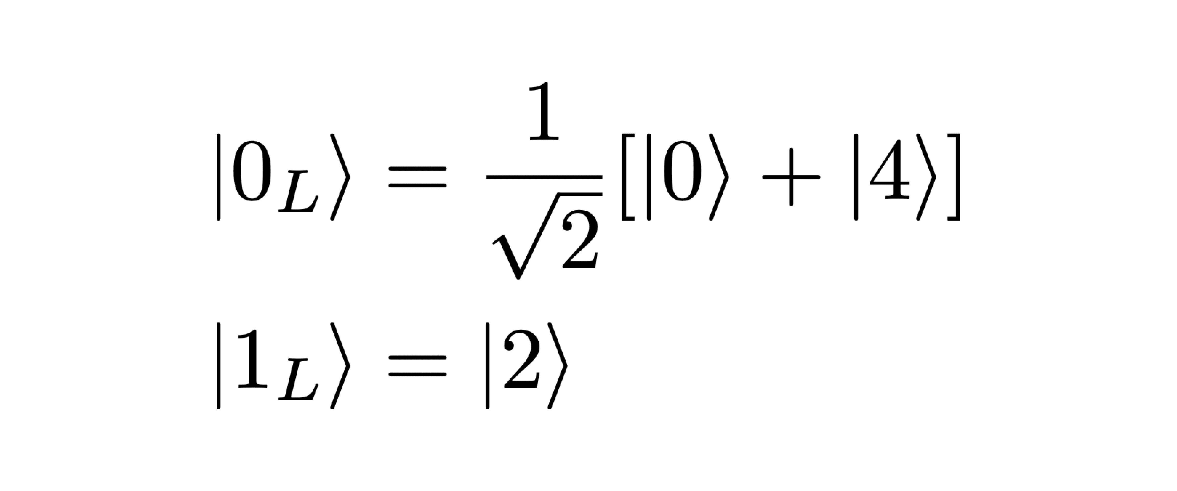
Beyond the property that single photon loss errors do not result in a logical error, there are a few additional advantages to defining our logical states as such.

First, the average photon number for both code words is two. As the average rate of photon loss for a qumode is proportional to the photon number, this rate will be the same in both code words. Crucially, this means it is therefore impossible to infer logical information based on the rate of photon loss detection.

Second, as both code words have even photon number parity, single photon loss errors will map the logical states onto odd parity Fock states (|1_L⟩ → |1⟩, |0_L⟩ → |3⟩), conveniently enabling the detection of single photon loss errors by measuring the photon number parity (i.e., whether it is even or odd). Importantly, this is done without learning the photon number. By extracting only the minimal information needed to detect errors, the logical information will be preserved.

Implementing the kitten code in Bosonic Qiskit

Now that we have a sense of how the kitten code works, let’s see how we can use it to simulate error correction by leveraging the built-in functionality of Bosonic Qiskit. In brief, we’ll need to implement the following components:

1. The photon-loss error channel (for simulating errors)
2. Measurement of the photon-number parity (for detecting errors)
3. Recovery operation (when an error is detected)

Below, we briefly highlight the various functionalities that support our simulations. Please refer to our Jupyter Notebook for further implementation details.

Photon loss

Photon loss is implemented using Bosonic Qiskit’s PhotonLossNoisePass(), which takes as input the loss rate of the mode. Here, we choose 0.5 per millisecond, corresponding to a lifetime of 2 ms — roughly speaking, the average amount of time that Fock state |1⟩ will “survive.” We model idling time between error correction steps using the cv_delay() gate.

Error detection

As previously discussed, we can detect single photon loss errors by measuring the photon-number parity. In practice, this is achieved via the Hadamard test, a technique that relies on phase kickback using an ancillary qubit. In particular, we can use a controlled-rotation operation of the form CR(π/2) = e^{-i(π/2)σ_za†a} such that final qubit state depends on the photon-number parity (see Figure 1).

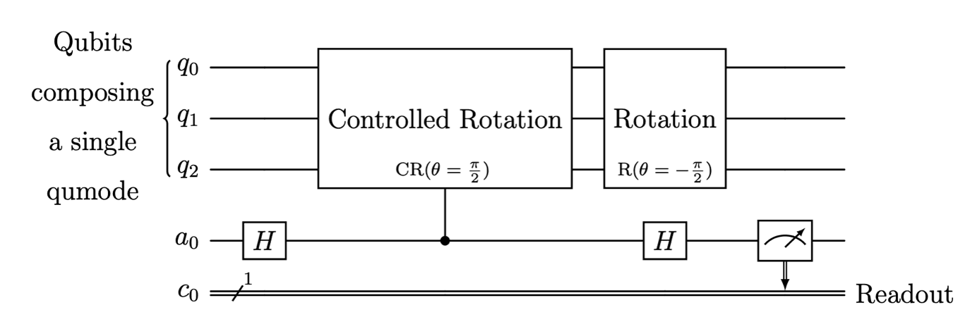
Figure 1: Circuit diagram for the parity check subcircuit. This subcircuit uses the Hadamard test to measure the parity of the qumode. The second uncontrolled rotation R(θ) = e^-iθa†a removes a global phase. As discussed in our previous blog post, Bosonic Qiskit represents a single qumode (with some cutoff) using a logarithmic number of qubits.

Recovery operation

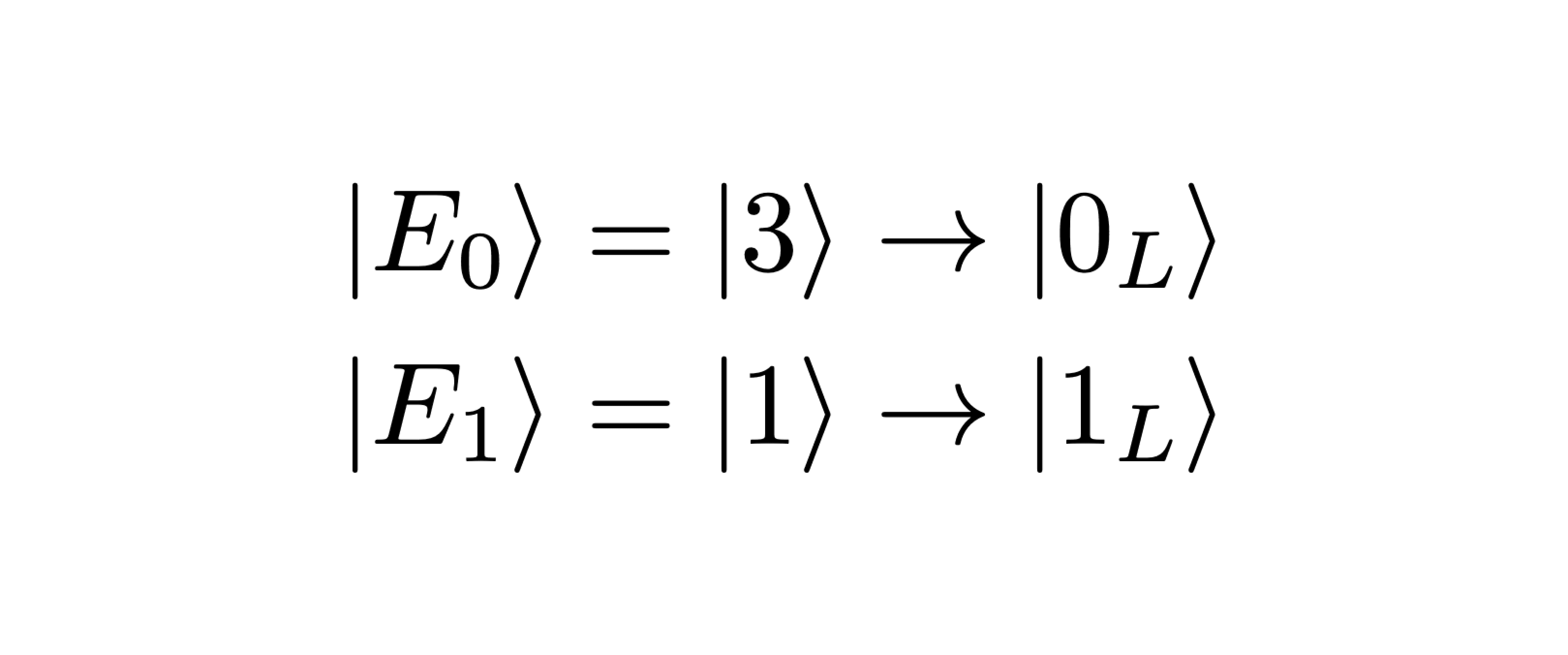
When an error is detected, we need to apply a correction that maps the system back onto the appropriate logical state. For the purposes of this tutorial, we will not go into detail on the specific sequence of gates needed to physically implement the error recovery operators for the binomial code. Instead, we will simply state the expected theoretical state transfer operation that maps the error states back onto our logical qubits.

If parity changes due to photon loss, the qumode will end up in one of two error states depending on the initial logical state: |1_L⟩ → |1⟩ ≡ |E₁ ⟩ or |0_L ⟩ → |3⟩ ≡ |E₀⟩. To correct the error state back to the logical state, we therefore require some unitary operation Û_odd that realizes the following mapping:

What if an error is not detected? You might guess that the answer is to do nothing, but this turns out to be incorrect. Quite non-intuitively, not detecting photon loss itself produces error!

To see why, imagine someone gives you a qumode prepared either in Fock state |0⟩ or |2⟩, and you have the ability to detect single photon loss through parity measurements. Now imagine that you repeatedly measure the parity over a timescale much longer than expected rate of photon loss, and keep finding that no photon loss has occurred. You might begin to suspect that the qumode is in the state |0⟩, and each repeated measurement will only enhance this suspicion.

In this way, even when the mode is in a superposition of |0⟩ or |2⟩, the state will decay toward |0⟩ through this phenomenon known as “no-jump backaction”. Consequently, we can further improve our error correction protocol by applying a correction Û_even that undoes this no-jump backaction when even parity is measured.

Putting it all together

Finally, we can put these components together to realize the protocol illustrated in Figure 2a. As this simulation does not include any other errors beyond photon loss, it is possible for us to achieve arbitrary enhancement by increasing the rate of error-correction. (Note: This would not be the case in a more realistic model where ancilla and gate errors are included. We’ve included the ability to add these additional error types as an option in the full Jupyter notebook).

In Figure 2b, we show the average fidelity of the initially prepared logical state |1_L ⟩ as a function of time for various error-correction rates. These results clearly demonstrate the expected trend that the lifetime of the logical state increases with the rate of error-correction.

Figure 2: Implementation of the binomial “kitten” error correcting code. (a) A circuit implementing the error correction cycle. Here, cv_delay(T) implements the error channel for chosen time T. The parity check (during which errors can also occur) is used to detect errors. Finally, we apply a recovery operation dependent on the outcome of this measurement. This cycle is repeated for 12 ms. (b) State fidelity averaged over 1000 shots as a function of time for various error correction rate. The no error correction case is shown in blue, while successive colors illustrate the (theoretical) improvement in lifetime enabled by error correction. To extract estimates of the error-corrected lifetime, we have fit exponential curves to each data set.

Try it yourself!

In this article, we have described the basics of the binomial “kitten” code and have illustrated how to simulate it using the built-in features of Bosonic Qiskit. For more details on the full implementation that includes additional options (such as inclusion of Û_even and ancillary qubit errors), we recommend that interested readers download the full Jupyter notebook, designed to be interactive such that users can generate error-correction simulations using parameters of their choosing.

For more information about Bosonic Qiskit, including installation instructions, see the GitHub repository. We particularly encourage new users to look at the tutorials and PyTest test cases. For those unfamiliar with bosonic quantum computation in general, we recommend the recently developed Bosonic Qiskit Textbook written by members of the Yale undergraduate Quantum Computing club Ben McDonough, Jeb Cui, and Gabriel Marous.

Bosonic Qiskit is a Qiskit ecosystem community project. Click here to discover more Qiskit ecosystem projects and add your own!